The relation between mass and time period for a spring Original teacher's comment:
"This is a model report which is not perfect, but should give an idea of what type of work is expected in the IB physics program."
|
Editor's initial comments This is a standard teaching lab that is well known. It is really not suitable for an IB intermal assessment unless something extra is attempted.
|
1. AIMS
1.1. Research question
We decided to experimentally find the relation between the time
period T (meaning the time to complete an oscillation, from one
extreme to the other and back) and the mass m attached to a given
metal spiral spring.
1.2 Hypothesis
While planning this lab we had access to the spring and a various
common lab equipment and we played a little with it. It seemed
that the heavier the object on the spring was, the slower would
it bounce up and down. We therefore make the hypothesis that
T will be proportional to m; or with a formula: T = km. Note
that k is here not the spring constant but just a constant we
define like this for now.
1.3. Variables
The variables we need to measure are the time period T and the
mass m attached to the spring. We are not sure if it makes any
difference how far we stretch the spring before releasing it.
2. METHODS AND TOOLS
2.1. Apparatus
To find the time period we used a digital stopwatch and to find
the mass we used an electronic scale. We also used a ruler to
measure the initial extension of the spring.
2.2. Control of variables
In case the initial extension of the spring would make a difference,
we used the same extension in all measurements. We were able
to take all measurements at one time, but we marked the spring
with a small piece of paper with our names taped to it in case
we would have had to repeat any measurements since there were
many springs that looked the same and we do not know if that
means they are all the same. Some may have been used too many
times and behave differently from a new spring.
2.3. The method used
We attached a chosen mass to the spring and secured it with a
small piece of tape, stretched it 3 cm and released it.
The stopwatch was started when the equilibrium was passed and
the time for three full oscillations were taken. Here one full
oscillation means the time from start to the upper extreme, down
to the lower extreme, and back to a situation where the mass
passes the equilibrium going upwards. We would have liked to
take the time for 5 or 10 oscillations but something (maybe friction
or air resistance) damped them very quickly.
This was then repeated 5 times for every mass, and 5 different
masses were used (one to five 50 g metal weights with hooks were
placed together on the hook at the end of the spring). The results
are given in tables 3.1.A. to 3.1.E in section 3.1. below.
3. DATA COLLECTION
3.1. Measurements and observations
The quick damping of the oscillations is an observation already
mentioned in 2.3. The masses used were weighed on an electronic
scale with the uncertainty Dm = 0.5
g (half the limit of reading, 1 g).
Table 3.1.A.: mA = 49g±0.5 g
Measurement nr
3T (s)
T(s)
Residual(s)
1
0.94
0.313
0.002
2
0.92
0.307
(-)0.004
3
0.91
0.303
(-)0.008 » 0.01
4
0.95
0.317
0.006
5
0.94
0.313
0.002
Average T = 0.311 s
Table 3.1.B.: mB = 100g±0.5 g
Measurement nr
3T (s)
T(s)
Residual(s)
6
1.33
0.443
(-)0.003
7
1.36
0.453
0.007
8
1.35
0.450
0.004
9
1.71??
-
-
10
1.31
0.437
0.009 » 0.01
Average T = 0.446 s
Here we note that measurement nr 9 gives an exceptional value,
which is excluded from the statistics as a probable outlier.
Table 3.1.C.: mC = 152g±0.5 g
Measurement nr
3T (s)
T(s)
Residual(s)
11
1.63
0.543
(-)0.006
12
1.67
0.557
0.008
13
1.70
0.567
0.018 » 0.02
14
1.61
0.537
0.012
15
1.62
0.540
0.009
Average T = 0.549 s
Table 3.1.D.: mD = 199g±0.5 g
Measurement nr
3T (s)
T(s)
Residual(s)
16
1.88
0.627
(-)0.010
17
1.95
0.650
0.013
18
1.97
0.657
0.020 = 0.02
19
1.86
0.620
(-)0.017
20
1.90
0.633
0.006
Average T = 0.637 s
Table 3.1.E.: mE = 252g±0.5 g
Measurement nr
3T (s)
T(s)
Residual(s)
21
2.10
0.700
(-)0.009
22
2.19
0.730
0.021
23
2.00
0.667
(-)0.042 » 0.04
24
2.17
0.723
0.014
25
2.18
0.727
0.018
Average T = 0.709 s
The residuals, that is the difference between a measurement value
and the average of them, are given in table 3.1.F where the largest
residual, approximated to one significant digit and estimating
the minimum uncertainty under any circumstances to be 0.01s,
for each of the masses mA to mE are used as the absolute uncertainties
DmA to DmE
. The average times for one oscillation for the five masses is
approximated accordingly.
Table 3.1.F.
m(g)
Tav(s)
Dm(g)
DTav(
(s)
49 0.31
0.5
0.01
100
0.45
0.5
0.01
152
0.55
0.5
0.02
199
0.64
0.5
0.02
252
0.71
0.5
0.04
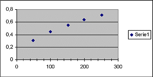
3.2. Presentation of the measurement results
To present the measurement results, with their uncertainties,
we plot Tav as a function of m (including
error bars in both dimensions) in graph 3.2.A below,:

Graph 3.2.A: Average oscillation time in seconds as a function
of oscillator mass in grams.
4. DATA PROCESSING AND PRESENTATION
4.1. Data processing
If the graph had been clearly linear, the students could here have moved on to find the proportionality constant they called k in section 2.2.. or alternatively just verbally stated that an inspection of the graph shows that it depicts a linear relation, since the research question strictly speaking is just to find the type of the dependency, not to determine a specific value. Ed.
We notice from the graph 3.2.A that the data do not seem to form
a straight line but some type of bent curve. Especially a line
from the origin to the first data point would not go through
the rest of them. We then tried to "linearize" the
graph by plotting some function of the variable T on the horizontal
axis. To make these graphs linear, we will first calculate the
values needed to plot T2 and
m with their error bars.
For the T2 plot, the values
of Tav in table 3.2.F are squared and
entered into the second column of table 4.2.A below. To find
the uncertainty in T2 we use
the formula (adapted from the IB data booklet)
D(T2)/T2 = DT/T
+ DT/T = 2DT/T
and then D(T2)
= 2T2DT/T
= 2T*DT
Example of one calculation: For the mass mA = 49 g, the
aboslute error is as before half the limit of reading or 0.5
g. For the average time of one oscillation we use T = 0.311s±0.01s
(see table 3.1.F). This gives T2
= (0.31 s)2 = 0.0961 s2. The error in this = D(T2) = 2T*DT
= 2*0.31 s*0.01 s = 0.0062 s2
» 0.006 s2. Thus we have
T2 = 0.096 s2
± 0.006 s2 which
is the first entry in table 4.2.A. below. The others in that
table are calculated in a corresponding way.
Table 4.2.A
m(g)
Tav2(s2)
Dm(g)
DTav2(s2)
49
0.096
0.5
0.006
100
0.203
0.5
0.009
152
0.30
0.5
0.02
199
0.41
0.5
0.03
252
0.50
0.5
0.06
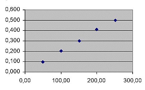
4.2. Presentation of processed data.
The values calculated in section 4.2. are presented in the following
graph (error bars in both dimensions).

Graph 4.2.A: The square of the average time for one oscillation
as a function of mass.
This appears to be a linear graph with the approximate gradient
0.50 s2 / 250 g = 0.50 s2 / 0.25 kg = 2.0 s2
kg-1.
5. CONCLUSION AND EVALUATION
5.1. Conclusions.
It seems that the hypothesis of a linear dependency of the form
T = km turned out to be wrong. The data would rather suggest
a formula of the type T2 =
km with k = 2.0 in SI-units. In the literature (reference: ......)
we have found that the formula should be:
... where the k represents the spring constant. An investigation
of the spring constant of the spring used could give more information
about whether or not our k-value is in accordance with this.
5.2. Evaluation of the procedures and results.
While taking the measurements we found that it was difficult
to say exactly when the mass oscillating on the spring was passing
its equilibrium - a place where more accurate time values can
be obtained than at the points of extreme displacement.
5.3. Suggested improvements.
To address the problem mentioned in section 5.2. we suggest that
the equilibrium level should be indicated by a marker line on
a paper directly behind the spring, or possibly with a laser
trained at that level adjusted so that the oscillating mass is
hit by the laser spot when it is at the equilibrium.