|
Random and systematic errors (uncertainties) Random errors due to many sources and are distributed in a normal distribution. Systematic errors due to a single factor that is the same for each trial have a single value. If a ruler is wrong then any measurements of a length will be wrong by the same factor before any random errors occur. Systematic errors are difficult by their very nature for students (and professional scientists) to quantify and are usually neglected in student work. Questions 1 Specific heat measurements by the method of mixtures are plagued by 20-30% heat losses. Are these losses systematic or random. Argue the case. 2 The latent heat of melting of ice can be determined by supplying electrical power to a calorimeter containing ice and water at zero degrees Celsius. If two different power settings are used the heat losses can be factored out of the calculations. a Show this. b Explain why this is possible in principle for any determination of a specific latent heat. 3 What follows in the body of this article applies to random errors only. Explain why. |
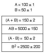
Uncertainties propagate through calculations. It is always possible to perform an extreme values calculation to find a final uncertainty.
1 Calculate an answer using the absolute values.
2 Calculate an answer that is as different as possible, given the stated uncertainties.
3 Write down the difference between 1 and 2 as the uncertainty and round to the appropriate number of significant figures.
For instance:

Round uncertainties to one significant figure. Reduce the figures in the absolute value to match the error. Upper and lower limits are usually the same to one significant figure ... or nearly so.
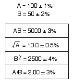
If errors are small it can be shown that the error in a product is the sum of the percentage errors.

Round percentage errors to one significant figure. It would be silly to write ...
The answer is written as ...
| Remember - the percentage error rule should only be used with small errors of a few percent and it only applies to products, powers etc. For large errors and for math functions, sines, cosines, logs etc. it is more reliable and more efficient to make an extreme value calculation to find a final uncertainty. |
Sample error calculations
Good research reports at IB level contain sample error calculations, so that the reader is explicitly made aware of the student's competence and understanding.
There are three simple steps to an error calculation.
1 Find the value without errors.
2 Find the largest possible value.
3 The error is the difference.
Sample error calculations that students put in research reports are often strictly correct ,but clumsy. Use these examples as a guide.
Example 1 Double calculation in Logger Pro
Example 2 Extreme lines fitted by hand
Slope =130±(80-74.3)/0.040 = 130±10 cm Example 3 Double calculation in Logger Pro
Example 4 Double calculation in Logger Pro
Example 5 Percentage errors
Example 6 Average deviation (preferred)
Example 7 Standard deviation
Random errors are differences between measurements of the same thing taken at different times or by different people.
To reduce the effect of random errors several independent measurements are averaged.
Express a final value as ...
Six independent readings of a measured Y value are graphed at right. The student must now decide how to find the likely error in the average of the six values.
There are many ways of doing it. The error may be stated as....
1 ... half the range.
2 ... the mean range.
3 ... the average deviation.
4 ... the standard deviation.
|
Half the range (for three-four points) The quickest and easiest alternative is to write down the average value, and use half the range as the error. The range is 4 The problem with this approach is the increase in range with increasing numbers of points. The average is more accurate if more data are available - but the range becomes larger. |
|
Mean range (for four-six points) The error can be calculated as the range divided by the number of data points. The range is 4 There are six data points ... This method has the advantage of reducing the likely error as the number of points increases. |
|
Average deviation (for six-eight points) The average deviation is the sum of the deviations divided by the number of data points. The deviations are ... 2, 1, 0, 0, 1, 2 (S Deviations) / N = 6/6 The average deviation is a compromise between the two simpler methods and is preferred, unless there are more than ten to twenty points, in which case the standard deviation is often a better estimate. |
|
Standard deviation (for ten or more points) Standard deviation is the preferred likely error when there are ten or more data points. SD can be calculated from a fitted Gaussian function in Logger Pro, and/or can be found by noting the half-width of the distribution at half-height. Two out of three values in a normal (Gaussian) distribution lie within one standard deviation of the mean. To find the standard deviation for a set of values enter the values into Logger Pro, highlight the graph and go to Analyze - Statistics. |
Systematic errors occur when an instrument is wrongly calibrated or there is some unknown factor affecting all readings. If a ruler is wrong all measured lengths will be wrong. If there is and unknown quantity of salt in a sample of distilled water the conductivity will always be too high.
Systematic errors are not dealt with in simple lab exercises. Rulers could be checked with gage blocks but the time and expense are not considered worth the effort in teaching laboratories. Students may assume that a manufacturer will not put marks on a scale that are meaningless. Analog meters and rulers are to be taken as accurate to within half the smallest scale division. The booklet that comes with digital meters contains information on the accuracy to be expected on different ranges.
Logger Pro includes a Gaussian distribution function and a normalized Gaussian in the curve fit options. These curves can be fitted to a histogram as visual confirmation of the statistical calculation of a standard deviation.
The Gaussian function has the form ...
Inserting appropriate constants ...

... where s is the standard deviation (half width at half height).
A final random error is normally the combination of many small independent errors, positive and negative, and of similar relative magnitudes. In this case, it can be shown that the distribution of values is Gaussian. [Interested readers should consult a reference to the Central Limit Theorem]. When errors are not strictly distributed in this way a Gaussian distribution is an appropriate approximation, because errors are determined approximately to one significant figure, and it is important to have a function for which an approximate standard deviation can be easily calculated.
An example of the Central Limit Theorem
Many people seem to believe that the accuracy of a stopwatch is limited by human reaction time, which is around 0.2 seconds. That is not true when measuring the period of a pendulum, as a student can verify for themselves. It is possible to obtain consistent times to within ± 0.04 seconds or less with a little practice.
Reaction time can be measured with the tester included here.
